Introduction

This section of the help guide explains some concepts and tips on how to import projections from other websites or electronic sources into the Cheatsheet Compiler. The need for this guide has mostly been replaced with the introduction of Projection Pal, but this information can still be useful for some tasks. Projection Pal is available as a separate download from the member access page.

Importing Projections

Lets input the above projections in the Compiler section Site B. Go to the qb tab, cell DV5. This is the top line on the QB tab under the column PaYd. The formula in this cell should be (using our example):

=VLOOKUP($C5,Sheet1!$A$2:$D$3,2,FALSE)

$C5 is finding the player name in the Compiler the formula will look for in the new projection table

Sheet1!$A$2:$D$3 is the table reference for the new projections.

2 is the column number we want to pull data from in the new projections table, 2 being PaYd, the second column over in our table reference above.

FALSE makes sure the VLOOKUP formula looks for an exact match in the name. This makes sure it doesn't grab projections from the wrong player if he isn't in the list or if the name is spelled wrong.

Now, once this formula is in place, you can copy it across to the other stat categories in Site B, but you'll have to go back and change the '2' to the appropriate column reference for each stat category. From our example, the formula for PaTD should be:

=VLOOKUP($C5,Sheet1!$A$2:$D$3,3,FALSE)

and for RuYd:

=VLOOKUP($C5,Sheet1!$A$2:$D$3,4,FALSE)

...because these are the column numbers we find these stats in our new projections table.

At this point, we have the proper formulas in the top row of the Compiler. Now copy these formulas down through Site B. It should start picking up stats for all players it finds in the new projections table. For every player where there is not an exact match of player names, it will return #N/A, which is ok.

Now, do some checking that the stats came over properly. At this point we don't want those formulas in there anymore. Highlight the entire Site B stats. Choose Edit > Copy or right-click Copy. Without moving the cursor anywhere, we are going to copy the same thing on top of itself, but paste it as values to get rid of the formulas. Choose Edit > Paste Special.. As Values.

I know this seems long but once you get the hang of using VLOOKUP, it really isn't so bad. Delete all the cells showing the #N/A because they had no match. A quick way to do this is to use Find and Replace options in Excel (Edit > Replace).

Finally, you have projections in Site B without typing them all in.

Formatting Player Names

From above, I skipped over the part about getting player names to the same format between the new projection table and the Compiler, but this is a crucial step if they are not already conveniently the same (unlikely).

If you copy projections off a website, then they can probably be in a few different forms, like:

The first one in the list is great because that is the way names are inputted in the Compiler. Any of the other ones we need to do some work.

1. Data > Text to Columns..

In number 2 in the list above, the First Name and Last Name are in the wrong order, and separated by a comma. So we need to take a couple steps here to get to what we want, the formatting in number 1, above.

First, we need to split apart the name into 2 columns. Insert a blank column beside the player names column. Then highlight all of the player names and choose Data > Text to Columns.. from the menu.

At this point it gives you two choices, Delimited and Fixed Width. We want Delimited. Choose this and hit "Next". Since we have a comma between the First and Last Name, that is the delimiter we want. Choose the "comma" checkbox. You should see an example of the data splitting into 2 columns.

Hit "Finish" and now the names should be in 2 columns. Still not what we are looking for but we're getting there. Which leads me to...

2. CONCATENATE function

What this does is combines cells, text, etc. into a single cell. We're going to combine the cell holding the player's First Name and the cell holding the player's Last Name, plus put a space between first and last names.

Say we now have the following:

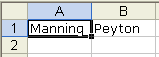
In our example, we're going to put the following formula in cell C1:

=CONCATENATE(B1," ",A1)

This will result in "Peyton Manning", which is cell B1 + a space + cell A1.

Copy this formula down for all players. Now, similar as mentioned above when importing projections, we want to eliminate the formulas and just have the values. Highlight and copy the player names created from the CONCATENATE functions. Then in exactly the same spot, choose Paste Special.. As Values.

At this point you're effectively turned Manning,Peyton into Peyton Manning and are ready to apply the VLOOKUP functions.

In the examples above where the names are already in 2 columns you won't have to worry about splitting the name. Just apply the CONCATENATE concepts and you should be good to go.

3. Edit > Replace

In number 3 in the list above, the First Name and Last Name are in the wrong order, and separated by a comma, but there is also a space in there will throw us off. Remember, it has to be exact.

We can quickly fix this though. Just highlight all of the names in your new projections table, choose Edit > Replace from the top menu. In the "Find" box just put one space " ". In the "Replace" box, don't put anything. Hit the "Replace All" button and it should quickly get rid of those spaces in the cells that were highlighted.

One thing to be careful of is of players with more than just that space before the comma. If they have 3 names (Randle El, Antwaan) then the replace will slam the Randle and the El together (RandleEl) which isn't right. Just watch out for things like that, but it is pretty rare.

Another thing to be aware of (and this is really tricky), is that sometimes what looks like a space on the Web is actually another special character that represents a space. So even though it looks like a space, it is actually something else, and two apparently identical player names will in fact not be the same.

What you need to do in this case is replace the special character, likely with a real space. To capture the special character, with your mouse highlight the spot where you think it is (between the first and last names), hit CTRL-C to copy it, and in the "Find" box paste it into the box by hitting CTRL-V. Input a real space in the "Replace" box, and follow the other steps as noted above and you will have effectively eliminated that special character.

After this, then you can apply the steps using Data > Text to Columns.. and CONCATENATE functions to get the desired naming format.

4. P. Manning

This one is a problem. Obviously no Excel functions or features are going to fill in missing characters in a name. But, if you have a situation like this, maybe you don't want to do VLOOKUP at all but rather use copy and paste. Let me give some hints and warnings on potential traps with that in my next post.

Copy & Paste, Drag-and-Drop

Here is a completely different way of getting projections in the Compiler, again without retyping them.

You have your table of new projections in a blank sheet. What we are going to do is copy them into the Compiler. Wait a second though, because there are some precautions/steps that need to be taken or we're sure to screw up the formulas that calculate the FF Pts.

First, the projections we are going to copy in should be in the same order as they will be in the Compiler. That is, for QB it should:

Plus the player name will be in the first column. If the projections you copied don't include some stats (like PaComp or 100+RuYd), then include a blank column in your new projections where those stats would otherwise be.

It is almost time to copy them over. First though, we want to insert a blank column beside where we are putting the new projections in the Compiler to temporarily hold each players name. This will help us line up the correct projections with the correct player in the Compiler. Say we are inserting QB projections in Site B of the Compiler. Insert a blank column in column DS (highlight DS and right click Insert and choose Entire Column).

Now we're ready to copy the new projections over. Highlight the new projections, choose Edit > Copy and go to the Compiler. Place the cursor on the top left corner of the space where the new projections will go. Try to keep the formatting of the numbers by choosing Edit > Paste Special.. As Values rather than a straight paste.

The new projections are in there now, but they probably aren't lined up with the correct players as shown on the left of the screen. Time to use drag-and-drop.

For each player highlight there name and new projections under Site B. Then place your mouse cursor near the edge of the box until an arrow appears. When this happens, hold down the mouse button and you can move (drag) the cells to a new spot. Line it up with the player name from the Compiler and release the mouse button to drop it in place.

Think of this as a puzzle. You might need to move some players out of the way before you can move new players in the right place. Or, if some players are in the same order, you can move a bunch at one time.

The biggest precaution with drag-and-drop is it will mess up the formulas. What I suggest is to never drag-and-drop anything in or out of the top player row. That way the formulas in that top row should never be disrupted. Once all of your other drag-and-drop is done, copy all the formulas in row 5 from column I all the way to column AI down over all the other players. That should correct any problems that occured from drag-and-drop.

Questions?
Check out the Compiler Message Board or send an email to Mike MacGregor and he will respond ASAP.